
Pioreactor development log #4

🌊 This week we investigated some sampling tricks to improve our ADCs, and managed to get a 50% reduction in signal variance, and gain many more bits in our signal, using data science!
In our development boards, we are using the terrific ADS1115 chip to convert our analog optical density signal into digital format that our Raspberry Pi can read. The ADS1115 is a high quality chip: 16-bits (meaning it can output any integer between 0 and 65535), has a programmable gain, and programmable samples-per-second (SPS). Unfortunately, it's also pretty expensive - up to $9 / chip. That's by far the costliest piece on our boards. Fortunately, there is a cheaper chip from the same family: the ADS1015. It's half the price, has 12-bits, and same programming. To make the Pioreactor as affordable as possible, we've done some evaluations and decided to move to the ADS1015.
However, the ADS1015's minimum SPS is much higher - 16x higher. Internally, a lower SPS means that the ADC can smooth over noise and produce a lower variance output. A higher SPS means a nosier output, but we can sample faster and perform some aggregation of those samples. So by moving to the ADS1015, we require our software to i) sample faster than currently, ii) perform an aggregation on the sequence samples to reduce the noise.
We wanted to maintain a reporting frequency of an OD measurement every 5 seconds. So, every 5 seconds, we sample the ADS1015 25 times over a one second interval. We then aggregate these 25 samples into a single optical density to report. The aggregation we chose was the sample average.

Quick note on a source of noise in our system. We observed early on that for very small signals, we were picking up a 60 hz signal caused by nearby AC (really it was common mode current). This resulted in strange "wave" behaviour that was really an aliasing artifact of sampling at ~0.2 hz.
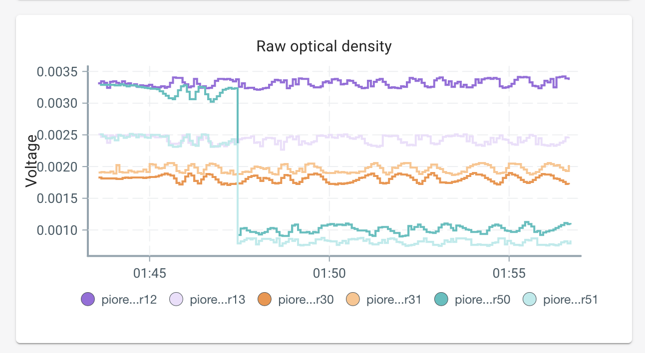
Figure 2. Some trial data showing patterns caused by aliasing of a nearby 60 hz signal.
We have some upcoming hardware solutions to reduce it, but they will not eliminate it. For strong signals, this artifact is still there, just a lot less significant. However, when the user starts an experiment and the cell density is low, this pattern shows up.
During some debugging of the optical density sampling code, I started thinking about about our choice of the sample average as our aggregation function. Maybe the average wasn't best - maybe something like a trimmed average would be better? Or maybe the median? Would another aggregation function have less variance for our data?
I ended up plotting the 25 samples, and was kinda surprised (at first):

I realized what was going on: aliasing. Again, a nearby AC current was creating a 60 hz signal, and I was sampling at well below 60 hz, creating this periodic artifact. But, this gave me confidence that the sample average certainly wasn't optimal. Consider the four situations, each equally likely: the initial sampling starts high / low, the end of sampling ends high / low. When both are high & high, the sample average over-estimates. When both are low & low, the sample average under-estimates. Now, on average, the errors cancel out, but this implies that the variance is higher than it could be. A better estimate, which wouldn't have the problem above, is to determine the constant value that the signal fluctuates around (the DC offset).
Formally, I can model the sequence of signals as a non-linear sinusoidal regression: $$ f(t_i; C, A, \phi, \omega) = C + A \sin(2\pi\omega t_i + \phi) + \epsilon_i$$ where \(t_i\) are the times I sample at, \(C, A, \phi, \omega\) are unknown parameters, and \(\epsilon_i\) is an error term. Really, the value I want is just \(C\), the offset term, but I need to solve for all of them to know \(C\). As is, this regression is difficult: it's non-linear (so requires more advanced solvers), is multi-modal (so solutions are not unique), and has a low data points / parameter ratio. We actually know the value of \(\omega\) though: it is produced by a 60 hz signal (50 hz in other parts of the world) - so we can fill that in right away. $$ f(t_i; C, A, \phi) = C + A \sin(2\pi 60 t_i + \phi) + \epsilon_i$$ This radically simplifies our problem, as we can use a trig. identity to modify this: $$ C + A \sin(2\pi 60 t_i + \phi) = C + a\sin(2\pi 60 t_i) + b\cos(2\pi 60 t_i)$$ where \(A = \sqrt{a^2 + b^2}, \phi = \arcsin(b/\sqrt{a^2 + b^2})\). The latter equation is linear in its parameters, \(C, a, b\), which means we don't need fancy non-linear solvers anymore. In fact, the solution comes down to solving a system of three linear equations: wickedly fast!
Let's recap: we have a 25 sampled values from our ADC. We'd like an "aggregate" function that takes these 25 values and provides a single value, that also has low variance. Our 25 values have aliasing from a 60 hz signal. We used regression to fit a sinusoidal to the 25 data points to recover a good estimate of the offset, \(C\). This parameter, I argue, is a better aggregate of the 25 sampled points than using the sample average, as explained above. Below are the results of performing this regression for our example dataset presented in figure 3.

Figure 4. Our example data and the results of the regression, \(C = 1676.4, A=200.7, \phi=1.47 \)

Figure 5. Comparing the sample average to the regression's estimate of the baseline. Note that the sample average is likely underestimating, since both ends of the signal are low.
Early tests show that this new aggregation has reduced our OD signal variance by up to 50%. Figures 6 and 7 demonstrate the improvements:


Figure 7. Real data showing the previous strategy vs new strategy. The green line shows time of the deployment.
There are extensions to this new way of modelling our problem, too. For example, we can reduce the variance further, and "borrow" information from preceding regressions by adding priors to our unknown parameters.
Two other benefits arise: First, the value of \(C\) has much higher resolution than the sample average, so we aren't as constrained by a 12-bit ADC. Secondly, the noise problem of 60 hz AC is effectively eliminated. We will still implement a hardware solution to reduce the noise, but early tests show that by modelling the 60 hz signal in software, we have eliminated it from the output completely!